Contour lines

ggplot2

germansea

Y2025

In this blog post, we’ll explore how to plot contour lines from a raster using bathymetry data as an example.

Author

Miriam Lerma

Published

December 4, 2025

Intro

This months blog post is about how to create contour lines from a raster file, and how to add labels using the package shadowtext.

A contour line (also isoline, isopleth, isoquant or isarithm) of a function of two variables is a curve along which the function has a constant value, so that the curve joins points of equal value (Wikipedia).

In cartography, a contour line (often just called a “contour”) joins points of equal elevation (height) above a given level, such as mean sea level. A contour map is a map illustrated with contour lines, for example a topographic map, which thus shows valleys and hills, and the steepness or gentleness of slopes. The contour interval of a contour map is the difference in elevation between successive contour lines (Wikipedia).

Read

For the example, we will be using Bathymetry data. Bathymetry gives us information on the water depth around an area.

The data comes from: GEBCO: General Bathymetry Chart of the Oceans provides information from bathymetry in the ocean.

To download visit webpage. For more details and instructions on how to load bathymatry data in R go to my bathymetry post

Bath_0tif<-'https://github.com/MiriamLL/data_supporting_webpage/raw/refs/heads/main/Blog/2025/Bathymetry/gebco_2024_n60.0_s50.0_w1.0_e9.0.tif'

Load the terra package for reading raster data.

library(terra)

The function rast helps to read raster data, replacing package raster.

Bath_1raster<-rast(Bath_0tif)

Crop

Keep a reduced area for making the calculations faster.

ext(Bath_1raster)
crop_extent <- ext(3, 9, 53, 56)
Bath_2cropped <- crop(Bath_1raster, crop_extent)
plot(Bath_2cropped)

Contour lines.

Calculate contour lines. Since we are working with bathymetric data, and contour lines are often labeled with the prefix “iso-” based on the type of variable they represent, the lines derived from bathymetric data can specifically be referred to as isobaths.

Depth_range <- global(Bath_2cropped, fun = "range", na.rm = TRUE)
Depth_range

Contour_levels <- seq(0, -80, by = -5)

Bath_3contours <- as.contour(Bath_2cropped, levels = Contour_levels)

The resulting object class is “SpatVector”.

class(Bath_3contours)

Check by plotting the data.

plot(Bath_2cropped, col = terrain.colors(100), main = "Bathymetry 5m Contours")
lines(Bath_3contours, col = "blue")

Export the shapefile using the function writeVector.

writeVector(Bath_3contours, "Bathymetry_10m_contours.shp", overwrite = TRUE)

The contour lines are also available to download here.

Plot

Load the package sf to transform from SpatVector to sf.

library(sf)

From SpatVector to sf.

Bath_4lines <- st_as_sf(Bath_3contours)

Load ggplot2 to use geom_sf.

library(ggplot2)

Lines

Bath_5df <- as.data.frame(Bath_1raster, xy = TRUE)

library(tidyverse)

Bath_6sub <- Bath_5df  %>%
  filter(x > 2 & x < 10)%>%
  filter(y > 52 & y < 57)%>%
  rename(Bathymetry=3) %>%
  filter(Bathymetry < 10)

Bath_7centroids <- Bath_4lines %>%
  group_by(level) %>%
  summarise(geometry = st_centroid(st_union(geometry)))

Bath_8plot<-ggplot() +
  geom_raster(data = Bath_6sub , aes(x = x, y = y, fill = Bathymetry)) +
  scale_fill_viridis_c(option = "mako")+
  geom_sf(data = Bath_4lines, color = "grey", size = 0.3) +
  geom_sf(data = GermanNorthSea::German_land , color='#ffffbe', fill='#ffffbe')+
  geom_sf_text(data = Bath_7centroids, aes(label = -level), 
               inherit.aes = FALSE, size = 4, color = "white") +
  theme_void() +
  coord_sf(xlim = c(3.3,8.8),
           ylim = c(53.2,55.8),
           label_axes = list(left = "N", bottom = 'E'))+
  theme(legend.position = 'none')
Bath_8plot

Shadows

To be able to better see the text use the package shadowtext.

library(shadowtext)

Bath_7centroids_df <- cbind(Bath_7centroids, st_coordinates(Bath_7centroids))

Bath_9plot<-Bath_8plot+geom_shadowtext(
    data = Bath_7centroids_df,
    aes(x = X, y = Y, label = -level),  # label is -level to not show negative values
    size = 4,
    color = "black",
    bg.color = "white",   # white shadow
    bg.r = 0.15,          # radius of the shadow
    inherit.aes = FALSE
  )
Bath_9plot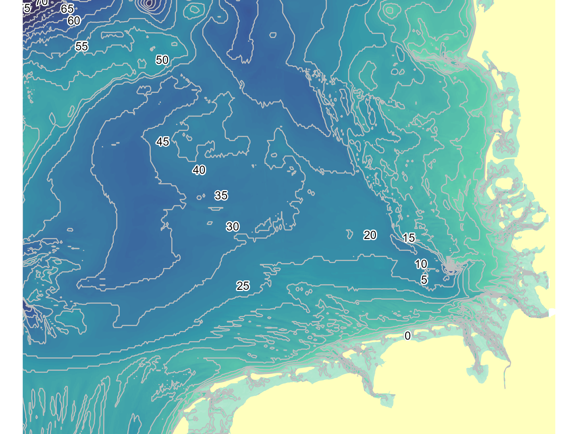

Other options

library(scico)

ggplot() +
  geom_sf(data = Bath_4lines, aes(color = level), size = 0.3) +
  scale_color_scico(palette = "imola", direction = 1) +
  geom_sf(data = GermanNorthSea::German_land, color = 'grey', fill = 'grey') +
  theme_bw() +
  coord_sf(
    xlim = c(3.3, 8.8),
    ylim = c(53.2, 55.8),
    label_axes = list(left = "N", bottom = 'E')) +
  theme(legend.position = 'right') +
  labs(color = "Depth (m)")