this_folder<-here()
this_file<-paste0(this_folder,"/GMT_intermediate_coast_distance_01d.tif")
this_raster<-rast(this_file)Distance to coast
r
ggplot2
germansea
Y2025
In this blog post, I share a step-by-step guide on how to use raster data from distance to the coast. I walk you through the steps I used using the North German Sea as an example.
Intro
Distance to coast gives us information on the distance (in meters) from one point at sea to the nearest coast.
This post includes:
- Download raster data
- Read and subset raster data
- Plot raster data
Distance to coast
To download:
- Access OceanColor NASA
- Select the interpolated 0.01-degree GeoTiff packed together with a brief description file.
- Unzip information.
Read and subset
To read from file.
Select the directory where the information is.
Alternatively, use the data directly from the repository.
DistCoast_tif<-"https://github.com/MiriamLL/data_supporting_webpage/raw/refs/heads/main/Blog/2025/DistanceToCoast/Subset_GMT_intermediate_coast_distance_01d.tif"Use the package terra to use the function rast.
Then convert to data frame.
library(terra)
DistCoast_file<-rast(DistCoast_tif)
DistCoast_dataframe <- as.data.frame(DistCoast_file, xy = TRUE)The file is quite large, so I recommend to subset the data to the area of interest.
Here I select the area close to the German North Sea.
library(tidyverse)
DistCoast_dataframe_sub <-DistCoast_dataframe  %>%
  filter(x > 2 & x < 10)%>%
  filter(y > 52 & y < 57)%>%
  rename(Dist=3) %>%
  mutate(Dist = as.numeric(Dist))
To save as rda would make the reading a lot faster.
German_distancecoast<-DistCoast_dataframe_sub
save(German_distancecoast, file="German_distancecoast.rda")
Plot
To plot adding land.
library(sf)Make sure is in the same CRS.
German_land<-st_transform(GermanNorthSea::German_land, 4326)To exclude information on land.
library(tidyverse)DistCoast_dataframe_sub<-DistCoast_dataframe_sub %>%
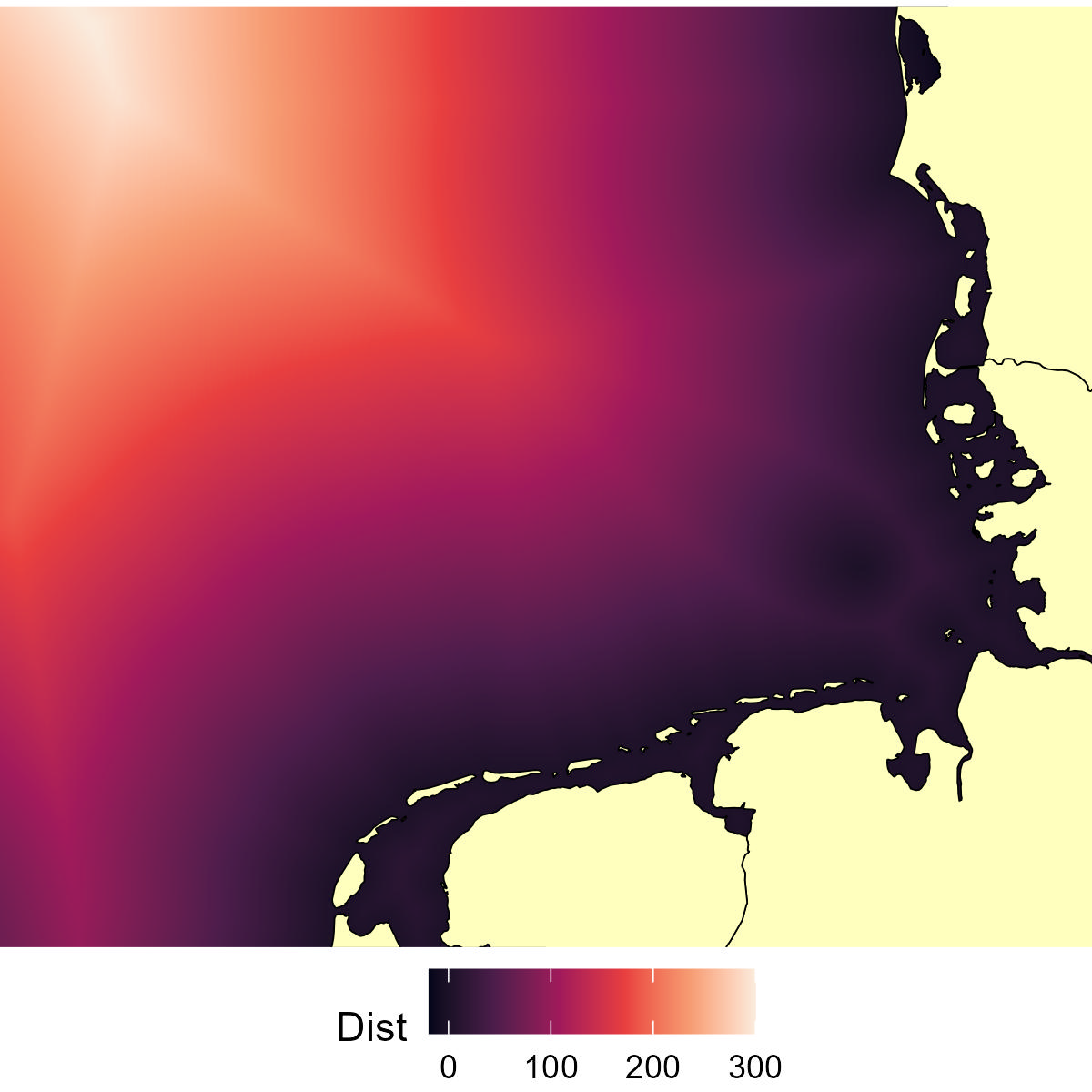
filter(Dist > -20)Use ggplot to create your plot.
Plot_distance<-ggplot() +
  geom_raster(data = DistCoast_dataframe_sub, aes(x = x, y = y, fill = Dist)) +
  geom_sf(data = German_land, colour = 'black', fill = '#ffffbe')+
  scale_fill_viridis_c(option = "rocket")+
  theme_void()+
  theme(legend.position='bottom')+
  xlab('Longitude')+ylab('Latitude')+
  coord_sf(xlim = c(3,9), ylim = c(53,56),
                    label_axes = list(top = "E", left = "N", bottom = 'E', right='N'))
Plot_distance+
  guides(fill=guide_legend(title="Distance to coast"))