Identify events

Assign a number to each event.

Intro

This post shows an option to assign a trip number to locations of animals.
This same method could be use to identify events on spatial data.

Data

For the exercises, test data is from Masked boobies.

#devtools::install_github("MiriamLL/sula")
library(sula)

This data frame contains data from 10 individuals.

unique(sula::GPS_raw$IDs)

Using functions from the package tidyverse, one of the individuals can be selected.

library(tidyverse)

GPS_one<-GPS_raw %>% filter(IDs=='GPS08')

The original data can be checked using functions from the package ggplot2.

library(ggplot2)

In the plot all locations are presented, but events can not be identify yet.

Plot_original<-ggplot(GPS_one, aes(x=Longitude, y=Latitude)) + 
  geom_point()+
  scale_x_continuous(labels = function(x) paste0(-x, '\u00B0')) +
  scale_y_continuous(labels = function(x) paste0(-x, '\u00B0'))  +
  ggtitle('Tracking data')+xlab('Longitude')+ylab('Latitude')+
  theme_bw()+
  theme(
    legend.position='none',
    panel.background = element_rect(fill = '#edf2f4'),
    panel.grid.major = element_blank(),
    panel.grid.minor = element_blank(),
    panel.border = element_rect(colour = "black", fill=NA, size=1.5))
Plot_original

Remove central locations

An event would be defined as each time the animal leaves its central location.

The information about the central location is needed.

Central_location<-data.frame(Longitude=-109.4531, Latitude=-27.20097)

The locations are to be transform into spatial data.

GPS_spatial <- GPS_one
sp::coordinates(GPS_spatial) <- ~Longitude + Latitude
sp::proj4string(GPS_spatial) = sp::CRS("+init=epsg:4326")
GPS_spatial<-sf::st_as_sf(GPS_spatial)

The buffer function is explained in the previous post.
The function uses the central location to create a buffer.
A number “1” shows that the location is inside the 1 km buffer and an NA that is outside the buffer.
The information is added on a column in the data frame.

create_buffer<-function(central_point=central_point, buffer_km=buffer_km){
  central_spatial<- sp::SpatialPoints(cbind(central_point$Longitude,central_point$Latitude)) 
  sp::proj4string(central_spatial)= sp::CRS("+init=epsg:4326") 
  central_spatial <- sp::spTransform(central_spatial, sp::CRS("+init=epsg:4326"))
  central_spatial<-sf::st_as_sf(central_spatial)
  buffer_dist<-buffer_km*1000
  central_buffer<-sf::st_buffer(central_spatial, buffer_dist)
  return(central_buffer)
  }
This_buffer<-create_buffer(central_point=Central_location,buffer_km=1)
GPS_over<-sapply(sf::st_intersects(GPS_spatial,This_buffer), function(z) if (length(z)==0) NA_integer_ else z[1])
GPS_one$trip <- as.numeric(GPS_over)

The NAs (when the animal is outside the buffer) can be replaced for a 0.
This is not strictly necessary but facilitates the interpretation of the column.

GPS_one$trip[is.na(GPS_one$trip)] <- 0

Alternatively, text can be added.

GPS_one$trip <- gsub("1", "At_central_locations", GPS_one$trip)
GPS_one$trip <- gsub("0", "At_trip", GPS_one$trip)

Assign trip number

To assign the trip number, the first step was adding a new column with a sequential number.

GPS_one$sequential_number<-as.integer(paste(seq(1:as.numeric(nrow(GPS_one)))))

Afterwards, all the locations inside the central locations were removed.

GPS_trips<-subset(GPS_one, GPS_one$trip == "At_trip")

By removing the locations inside the central locations, we end up with gaps in the sequence number.
Here, I added a number of event everytime that the sequence was broken.

GPS_trips$trip_number <- (cumsum(c(1L, diff(GPS_trips$sequential_number)) != 1L))+ 1

In case there might be more than ten trips, adding more zeros using the function str_pad might be useful.

GPS_trips$trip_number <- stringr::str_pad(GPS_trips$trip_number ,  2, pad = "0")

For easier interpretation, text can be added.

GPS_trips$trip_number<-paste0("Trip_", GPS_trips$trip_number )

Using the function unique the number of events (or trips) can be checked.

unique(GPS_trips$trip_number)

Plot

The different events can now be easily observed by adding the argument color=trip_number in the plot.

Plot_trips<-ggplot(GPS_trips, aes(x=Longitude, y=Latitude, color=trip_number)) + 
  geom_point()+
  geom_point(data=Central_location,aes(x = Longitude,y= Latitude), 
             color="black", fill="black",shape=16,size=5,stroke=1.5)+
  theme_bw()+
  scale_x_continuous(limits=c(-109.7,-108.9),labels = function(x) paste0(-x, '\u00B0')) +
  scale_y_continuous(labels = function(x) paste0(-x, '\u00B0'))  +
  ggtitle('Trip number')+xlab('Longitude')+ylab('Latitude')+labs(color='')+
  theme(
    panel.background = element_rect(fill = '#edf2f4'),
    panel.grid.major = element_blank(),
    panel.grid.minor = element_blank(),
    panel.border = element_rect(colour = "black", fill=NA, size=1.5),
    legend.background = element_rect(colour = "transparent", fill = "transparent"),
    legend.position = c(0.12,0.75))
Plot_trips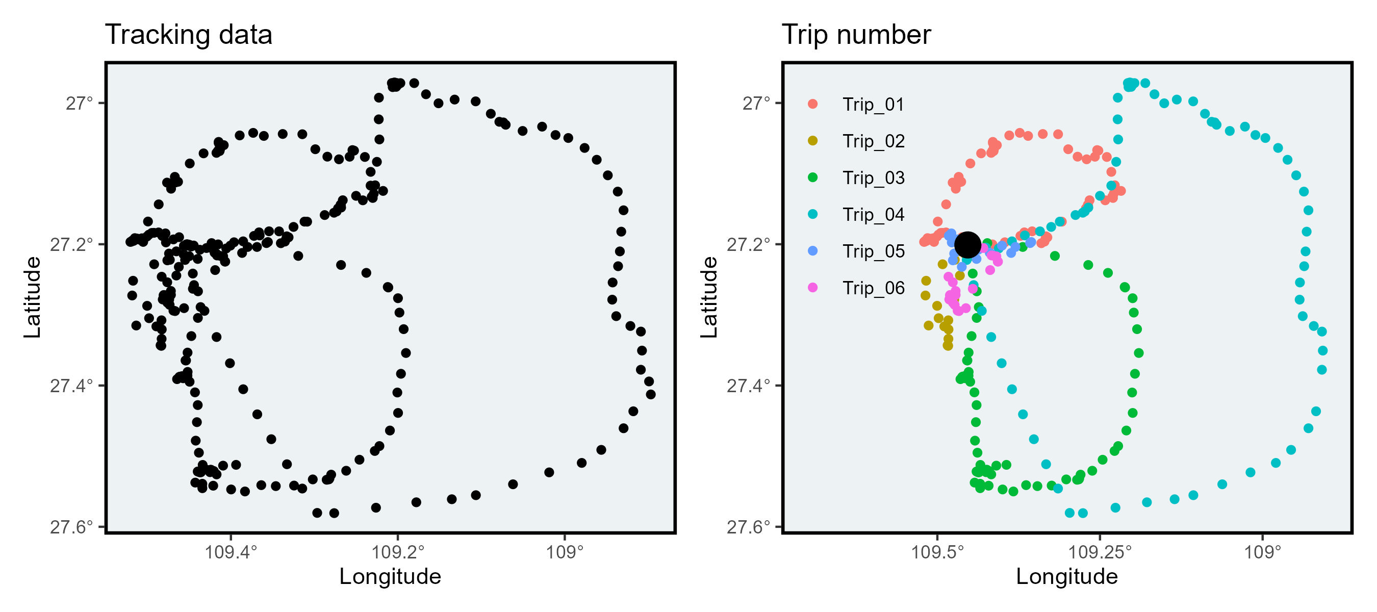

Further reading

Functions count_trips from the package sula can be used to run loops.