Remove undesired locations

Create a buffer to remove locations.

Intro

When studying animals using GPSs, we often need to remove their central location. Here, I am sharing a function I created to eliminate all the locations within an area.

Data

For the exercises, test data is from masked boobies.
To access the data you have to install the package sula: devtools::install_github(“MiriamLL/sula”)

#devtools::install_github("MiriamLL/sula")
library(sula)

This data frame contains data from 10 individuals.

unique(sula::GPS_raw$IDs)

To load it into the environment.

GPS_ten<-GPS_raw

Plot your data

library(tidyverse)

Here you can see all the recorded locations using the GPSs.

Original_plot<-ggplot()+
  geom_point(data = GPS_ten,
            aes(x=Longitude,y = Latitude),color='red', size=0.5)+
  scale_x_continuous(labels = function(x) paste0(-x, '\u00B0')) +
  scale_y_continuous(labels = function(x) paste0(-x, '\u00B0'))  +
  xlab('Longitude')+ylab('Latitude')+
  theme(
    panel.background = element_rect(fill = '#edf2f4'),
    panel.grid.major = element_blank(),
    panel.grid.minor = element_blank(),legend.position='none',
    panel.border = element_rect(colour = "black", fill=NA, size=1.5)
  )
Original_plot

Create a buffer

Select a location

This_point<-data.frame(Longitude=-109.5,Latitude=-27.2)

Create a buffer

I created this function to create a buffer around a point

create_buffer<-function(central_point=central_point, buffer_km=buffer_km){
  central_spatial<- sp::SpatialPoints(cbind(central_point$Longitude,central_point$Latitude)) 
  sp::proj4string(central_spatial)= sp::CRS("+init=epsg:4326") 
  central_spatial <- sp::spTransform(central_spatial, sp::CRS("+init=epsg:4326"))
  central_spatial<-sf::st_as_sf(central_spatial)
  buffer_dist<-buffer_km*1000
  central_buffer<-sf::st_buffer(central_spatial, buffer_dist)
  return(central_buffer)
  }

The parameters to give are the kilometers and the central point

This_buffer<-create_buffer(central_point=This_point,buffer_km=20)

class(This_buffer)

Here you can see the buffer you created using the point (or central location)

Buffer_plot<-ggplot()+
  geom_point(data = GPS_ten,
            aes(x=Longitude,y = Latitude),color='red',size=0.5)+
  geom_point(data=This_point,
             aes(x=Longitude,y=Latitude),color='blue')+
  geom_sf(data=This_buffer,colour='blue', fill='transparent', linetype='dashed')+
  scale_x_continuous(labels = function(x) paste0(-x, '\u00B0')) +
  scale_y_continuous(labels = function(x) paste0(-x, '\u00B0'))  +
  xlab('Longitude')+ylab('Latitude')+
  theme(
    panel.background = element_rect(fill = '#edf2f4'),
    panel.grid.major = element_blank(),
    panel.grid.minor = element_blank(),legend.position='none',
    panel.border = element_rect(colour = "black", fill=NA, size=1.5)
  )
Buffer_plot

Using the function from the package sp you can create an spatial object using your GPS data

GPS_sp <- GPS_ten
sp::coordinates(GPS_sp) <- ~Longitude + Latitude
sp::proj4string(GPS_sp) = sp::CRS("+init=epsg:4326")
GPS_sp<-sf::st_as_sf(GPS_sp)

class(GPS_sp)
class(This_buffer)

Here the function over identifies which location intersect with the buffer.

GPS_over<-sapply(sf::st_intersects(GPS_sp,This_buffer), function(z) if (length(z)==0) NA_integer_ else z[1])

This information can be added as a column in the data frame.

GPS_ten$In_or_out <- as.numeric(GPS_over)

To remove the locations that were within the buffer you can use the function filter and is.na from the package tidyverse

GPS_without <- GPS_ten %>%
  filter(is.na(In_or_out)==TRUE)

Here you can see that the locations inside the buffer were removed.

Filtered_plot<-ggplot()+
  geom_point(data = GPS_without,
            aes(x=Longitude,y = Latitude),color='red',size=0.5)+
  geom_point(data=This_point,
             aes(x=Longitude,y=Latitude),color='blue')+
  geom_sf(data=This_buffer,colour='blue', fill='transparent', linetype='dashed')+
  scale_x_continuous(labels = function(x) paste0(-x, '\u00B0')) +
  scale_y_continuous(labels = function(x) paste0(-x, '\u00B0'))  +
  xlab('Longitude')+ylab('Latitude')+
  theme(
    panel.background = element_rect(fill = '#edf2f4'),
    panel.grid.major = element_blank(),
    panel.grid.minor = element_blank(),legend.position='none',
    panel.border = element_rect(colour = "black", fill=NA, size=1.5)
  )
Filtered_plot

This function can be used to remove all the nest locations within a distance buffer. You could also replace the polygon (here the buffer) for some land shapefiles.

Compare

Using the package patchwork we can see the difference side by side.

library(patchwork)

Original_plot+Buffer_plot+Filtered_plot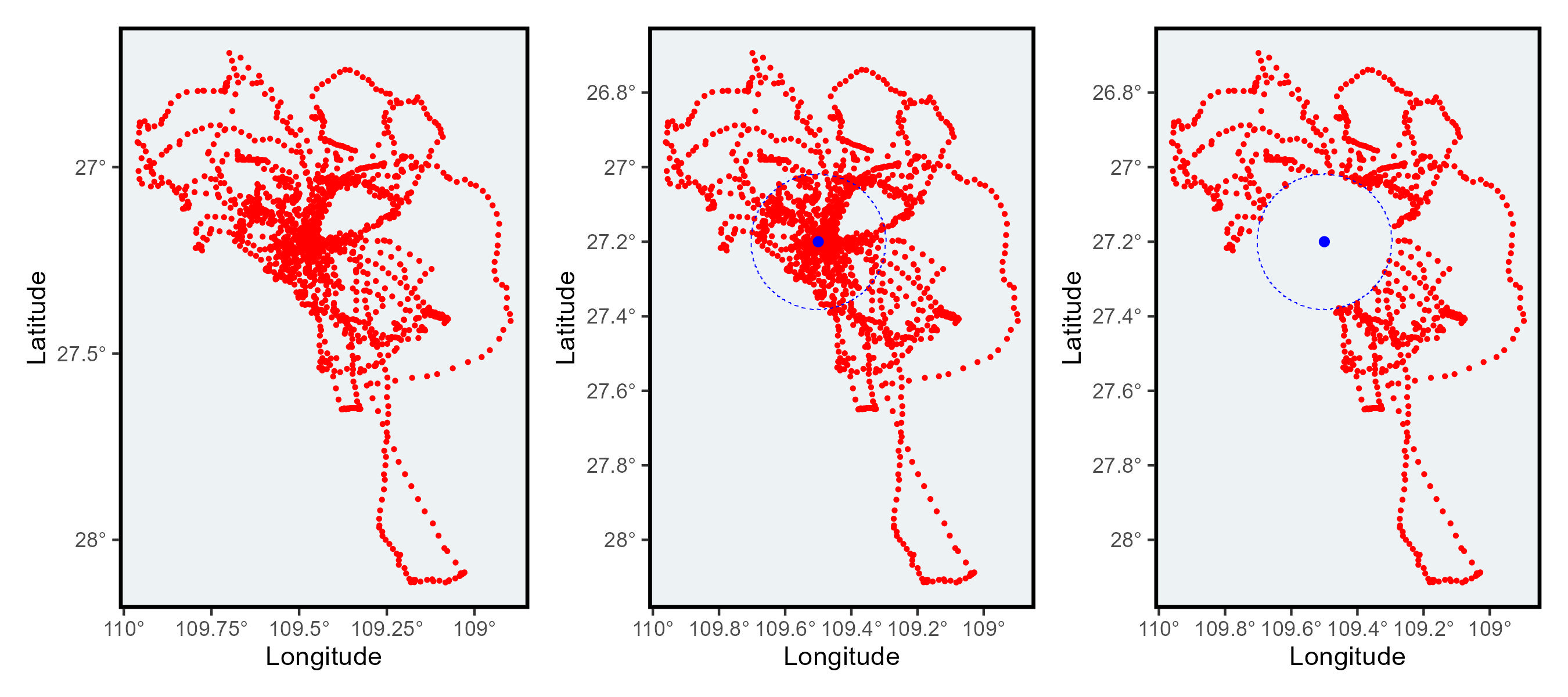

Further reading

Other functions that did the job:
gBuffer from rgeos deprecated
Read more about package sf