Grid, Raster, Colors

gis

Y2023

Create a grid, then a raster, and plot them with your custom colors.

Author

Miriam Lerma

Published

April 6, 2023

Intro

The goal of this post is to:

1- Create a grid
2- Extract values per grid
3- Keep only grid cells with values
4- Calculate mean values per grid
5- Customize raster plot

Data

For this example, we will use the data provided in the package sula
The data is from tracked masked boobies at Rapa Nui
The data is already in tidy format

my_data<-(sula::GPS_preparado)

Grid

Start by converting the data from data.frame to an sf object using functions from the package sf

library(sf)

Using the argument st_as_sf convert the data to a sf object

my_points<-my_data %>%
  st_as_sf(coords=c('Longitude','Latitude'),
           crs=4326,
           remove=FALSE)

For plotting the data use the package ggplot2

library(ggplot2)

Since the data is an sf object, use the function geom_sf to plot

ggplot()+
  geom_sf(data=my_points)+
  theme_minimal()

To create a grid using the points.

A common used method is the fish net. By definition, the fish net, or square grids, is a good method of covering a surface. The method is called tessellation, and it converts a surface with no overlaps or gaps, like when using tiles.

To create a grid the function st_make_grid can be used

The arguments of the function st_make_grid are:
n - an integer of length 1 or 2, which corresponds to the number of grid cells in x and y direction (columns, rows)
what - defines if polygons, corners or centers are to be created
square- is set to TRUE creates squares, if set to FALSE creates an hexagonal grid

To decide on the size of the grids, check the differences in latitudes and longitudes using the function range

range(my_points$Latitude)
range(my_points$Longitude)

my_grid<-st_make_grid(my_points, 
                       c(0.05, 0.05), 
                       what = "polygons",
                       square = TRUE)

Now that the grid has been calculated, transform the grid to sf using the function st_sf and add an grid_id to the grid cell using the function mutate from the package dplyr

library(dplyr)

my_grid_sf = st_sf(my_grid) %>%
  mutate(grid_id = 1:length(lengths(my_grid)))

To plot the recently created grid:

ggplot()+
  geom_sf(data=my_grid_sf)+
  geom_sf(data=my_points)+
  theme_minimal()

Extract values per grid

Using the function st_intersection the values from the points can be added to the grid

Using the argument lenghts the sample number per grid can be calculated

my_grid_sf$nlocs <- lengths(st_intersects(my_grid_sf, 
                                          my_points))

To add color to the plot, the package viridis provides the function scale_fill_viridis.

library(viridis)

The color will correspond to the number of locations (nlocs)

ggplot()+
  geom_sf(data=my_grid_sf,aes(fill=nlocs))+
  theme_minimal()+
  scale_fill_viridis(direction = -1)

Surveyed

To keep only the grid cells that were surveyed, the grid cells that have 0 recording can be removed

grid_w_data = filter(my_grid_sf, nlocs > 0)

To check which grid cells were removed, plot the previous and current grid

ggplot()+
  geom_sf(data = my_grid)+
  geom_sf(data = grid_w_data, colour = "#42a921", fill= '#bde0fe',alpha=0.9)+
  NULL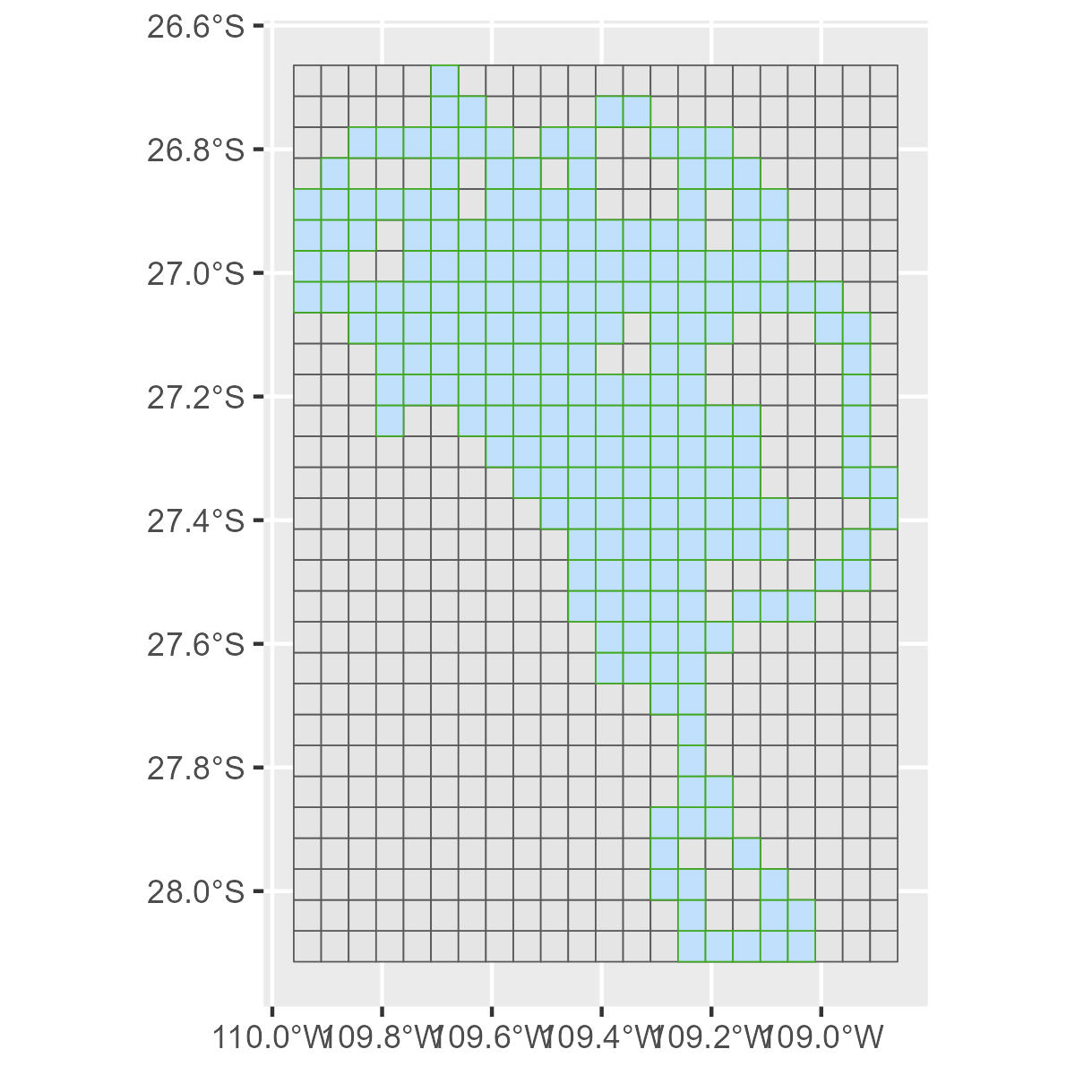

Mean values

To calculate the mean values per grid, functions from the package tidyverse can be used

my_dens<-my_points

For the exercise, generate random data using the function runif

my_dens$densities<-runif(nrow(my_dens), min=0, max=1)

To transform from data.frame to sf object the function st_as_sf can be used

my_dens_sf <-my_dens %>% 
  st_as_sf(coords = c("Longitude", "Latitude"))

To assign the coordinate system the function st_set_crs can be used

my_dens_sf  = st_set_crs(my_dens_sf , "EPSG:4326")

Using the function st_intersection, the grid number to each data point is added

dens_grid <- st_intersection(grid_w_data,my_dens_sf)

With the function mutate, the mean density per grid can be calculated

dens_mean <- dens_grid %>%
  st_drop_geometry() %>%
  group_by(grid_id)%>%
  mutate(grid_dens_means=mean(densities))

Finally, the mean density can be added to the general grid

grid_w_dens<-merge(grid_w_data,dens_mean, by='grid_id', all=TRUE)

There might be more than one value per grid, to have one value per grid the function summarise_at can be used.

grid_dens<-grid_w_dens %>%
  group_by(grid_id)%>%
  summarise_at(vars(grid_dens_means),
               list(name = mean)) %>%
  rename(dens_mean=name)

To remove grid without values, the function drop_na can be used

library(tidyverse)

grid_dens<-grid_dens%>%
  drop_na(dens_mean)

To check the values that were removed, plot the data.

ggplot()+
  geom_sf(data = grid_dens,aes(fill = dens_mean))+
  geom_sf(data= my_dens_sf)+
    scale_fill_viridis(direction = -1)

Customize

The function geom_sf allows to plot a raster

Axis labels can be changed using scale_x_continuous and scale_y_continuous

To see less distracting colors on the background, theme_minimal is a prefered option

ggplot()+
  geom_sf(data = grid_dens,aes(fill = dens_mean))+
    scale_fill_viridis(direction = -1) +
    scale_x_continuous(labels = function(x) paste0(x, '\u00B0', "W")) +
    scale_y_continuous(labels = function(x) paste0(x, '\u00B0', "N"))+
  theme_minimal()

To make a custom raster palette the function scale_fill_gradientn can be used

dens_colors<-c('white','#6CB4D3','#1A89AB','#7CC252','#B2EC2B','#DCF754','#FFE454','#FD9708','#F6640F','#EC2C11')
dens_breaks<-c(0,0.30,0.60,0.85)
dens_labels<-c('0','0.30','0.60','> 0.85')

The plot with custom palette arguments consider:
colours the number of colors should correspond to the values
breaks for those numbers that are to be displayed
labels for those labels that are to be displayed
limits to set up minimum and maximum values on the scale

To customize legend:
legend.key can be used

ggplot()+
  geom_sf(data = grid_dens,aes(fill = dens_mean),color='transparent')+
    
  scale_fill_gradientn(name='Density',
    colours = dens_colors,
    breaks = dens_breaks, 
    labels = dens_labels,
    limits=c(0,1))+
  
  
    scale_x_continuous(labels = function(x) paste0(x, '\u00B0', "W")) +
    scale_y_continuous(labels = function(x) paste0(x, '\u00B0', "N"))+
  
  theme_bw()+
  
  theme(panel.background = element_rect(fill = '#3668b4'),
        panel.grid.major = element_blank(), 
        panel.grid.minor = element_blank())+
  
  
  theme(
    legend.key = element_rect(color = "black",size=5),
    legend.key.width = unit(1, "cm"),
    legend.key.height = unit(1, "cm")) +
  
  guides(fill = guide_colorbar(ticks.colour = "transparent"))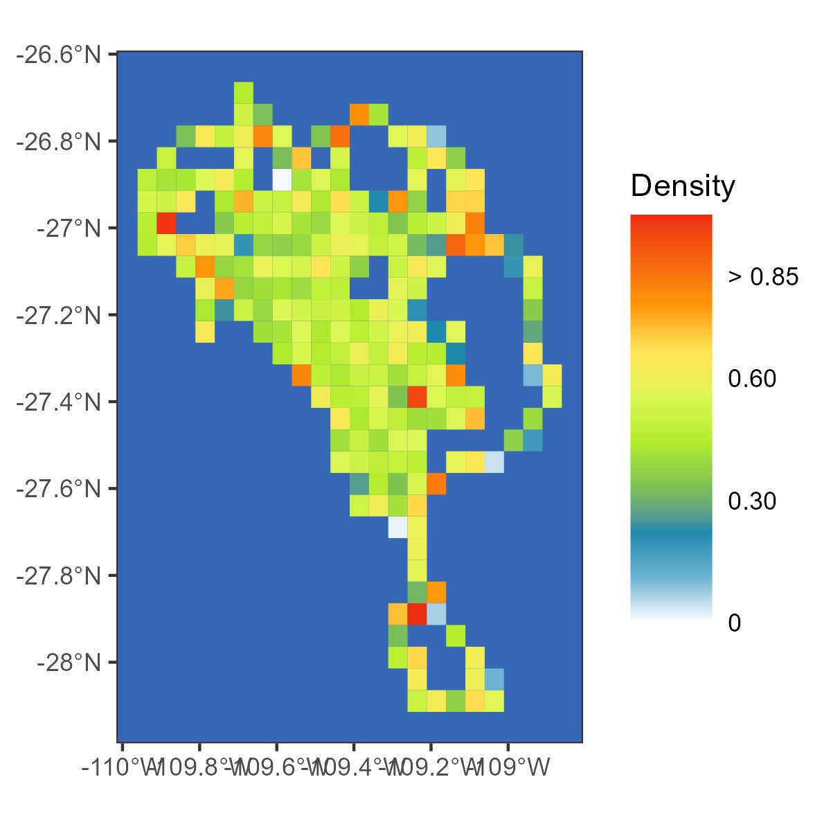