#devtools::install_github("MiriamLL/sula")Count days
r
biologging
sula
Y2022
How to add a day number as a column, and see differences as days pass.
Intro
This post is about how:
- Add a column counting the days (day 1, 2…).
- Check differences in parameters as days pass.
- Add a column with julian day (days from the first day of the calendar).
Examples
This post is useful to study:
In species that fed their offspring. Trips might be shorter when the parents need to mantain a constant feeding rate, but trips can be longer during the incubation period, and when offspring can be left unattended.
Species that use resources that availability change over time. Trips might be shorter when the prey availability is at its peak, and trips might be longer when the prey availability is lower, as individuals expend more time to reach their energetic demands.
Data 📖
To do this exercise, we will load data from the package ‘sula’
To install:
library(sula)To load data from from 1 tracked individual.
GPS<-GPS_editedGet nest location.
nest_loc<-localizar_nido(GPS_data = GPS,
                          lat_col="Latitude",
                          lon_col="Longitude")
Calculate foraging trip parameters.
Foraging_trips<-calcular_tripparams(GPS_data = GPS,
                              diahora_col = "tStamp",
                              formato = "%Y-%m-%d %H:%M:%S",
                              nest_loc=nest_loc,
                              separador="trip_number")
Count days 🧮
Ideally, you will have a data frame with the date and time information.
To add the number of days, we select a column with information from date and time.
For the example we will use trip_start and extract the date.
Foraging_trips$date<-substr(Foraging_trips$trip_start, start = 1, stop = 10)Now we use this date as a factor and number it.
Foraging_trips$day_number<-as.numeric(as.factor(Foraging_trips$date))We can also use this information to see the number of days the individual was tracked.
length(unique(Foraging_trips$day_number))Load the package tidyverse.
library(tidyverse)Summarize the information per day.
duration_per_day<-Foraging_trips%>%
  group_by(day_number)%>%
  summarise(duration_day=mean(duration_h))
In the plot, you can now see if there were differences in the trip durations among the days that the bird was tracked.
ggplot(duration_per_day, aes(x=day_number, y=duration_day)) +
  geom_segment( aes(x=day_number, xend=day_number, y=0, yend=duration_day), color="grey") +
  geom_point( color="orange", size=4) +
  theme_classic() +
  xlab('Days since begginnig of tracking')+
  ylab('Mean duration (h)')+
  scale_y_continuous(expand = c(0, 0), limits = c(0, 3))
Julian day 📅
Load package lubridate
library(lubridate)Extract the date using the function as.Date
Foraging_trips$julian_date <- as.Date(Foraging_trips$date, format=c("%Y-%m-%d"))Use the argument %j to obtain the julian day.
Foraging_trips$julian <- as.numeric(format(Foraging_trips$julian_date, "%j"))The bird was tagged between the day 306 and 309 of the calendar.
range(Foraging_trips$julian)Summarize the information per day.
duration_per_julian<-Foraging_trips%>%
  group_by(julian)%>%
  summarise(duration_day=mean(duration_h))
The plot would be more informative for whole seasons, or breeding seasons.
ggplot(duration_per_julian, aes(x=julian, y=duration_day)) +
  geom_segment( aes(x=julian, xend=julian, y=0, yend=duration_day), color="grey") +
  geom_point( color="orange", size=4) +
  theme_classic() +
  xlab('Calendar day')+
  ylab('Mean duration (h)')+
  scale_y_continuous(expand = c(0, 0), limits = c(0, 3))+
  scale_x_continuous(expand = c(0, 0), limits = c(0, 365))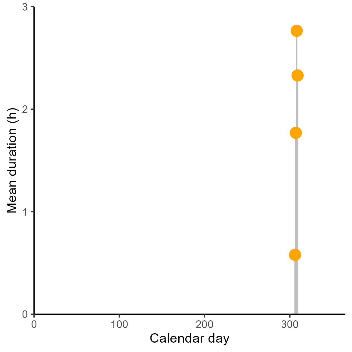
I hope this might help you.